Curve Fitting
Updated 12 November 2023
Introduction
When I joined Chemistry Division in the Department of Scientific and Industrial Research in 1974 I worked on Atomic Spectrometry with Dr. Reiner Goguel. This was mostly Atomic Absorption Spectrometry and Atomic Emission Spectrometry of solutions to determine their elemental composition. The working curves of concentration versus absorbance or emission were typically non-linear. There was reasonable linearity for small signals but as the amplitude increased, so did the non-linearity. This situation is not easily described by a simple function. For example, a certain commercial Atomic Absorption Spectrometer had a built in polynomial fitting routine for flame emission. For some flame emission signals negative concentrations were returned by this instrument.
For flame emission two processes occur. The signal amplitude grows linearly with concentration until the emitted signal reaches an amplitude matching that emitted by a black body at the emission wavelength and temperature. Spectral line broadening dominates after that as the black body temperature is never exceeded at any wavelength.
The first process tends to be linear while the second is parabolic.*
An Equation
Given the above information, a calibration equation is required which is linear for low concentrations and parabolic at high concentrations. To cater for other systems such as atomic absorption the second part of the equation was generalised to include a parabolic curve of any order. The following equation works and it found extensive use in our routine atomic spectrometry.
y is a concentration and x is the instrument signal reading.
y = a.xb + c.x.e-(d.x)
*The equation models the two features of typical flame emission curves outlined above.
The first term is a parabola of order b. The second term has a linear part multiplied by an exponential which reduces the effect of this term for large x. Possible values of the exponential factor range from 0 for large x to 1 for small x. It acts as a switch. No switching is necessary on the first parabolic term of the equation. The second linear part dominates at low x.
Four sets of readings are needed to solve this equation. x1 is typically a blank reading for y1 = 0.
For example:
- x1 = 0 (blank reading), y1 = 0 .. (blank concentration)
- x2 = 2 (std1 reading), y2 = 2 ... (std1 concentration)
- x3 = 4 (std2 reading), y3 = 5 ... (std2 concentration)
- x4 = 5 (std3 reading), y4 = 8 ... (std3 concentration)
- a = 1.194199E-04 .... (scale)
- b = 4.540601 .......... (order)
- c = 6.25E-01 ........... (slope)
- d = 6.553457E-03 .... (factor)
Before using the equation let xi=xi*10/x4
Normalising avoided exceeding the numeric range of programmable scientific calculators on certain data sets.
After using the equation let yi=yi*y4/10
- xi = 0, yi = 0.0000 ..... (Result 1)
- xi = 2, yi = 2.0000 ..... (Result 2)
- xi = 4, yi = 5.0000 ..... (Result 3)
- xi = 5, yi = 8.0000 ..... (Result 4)
It was the accurate fitting of experimental data that enabled this equation to be used routinely. For flame emission data the fit covered several orders of magnitude, provided the instrument slit width was wide enough - typically 5 nm for Na at 1000ppm. With narrower slits the useful concentration range is reduced. It was easy to make up intermediate standards to confirm the accuracy of the curve fitting. In most flame emission cases the order b of the equation was slightly greater than 2, as expected.
There may be several other equations that could be tried. Most are based on using an exponential term as a soft switch to gradually change from a linear equation to a parabolic form I was lucky that the equation above worked very well with my experimental data, so at the time I explored only a few other options.
Software
Several useful programs make up the AAFlame software collection:
- LINEAR - Linear fitting of data.
- DRIFT - Compensate linear data for drift.
- CURVE - Correct data for curvature.
- STRAY - Correct spectrophotometric data for the presence of stray light.
- BICURVE - CURVE and DRIFT combined.
- ABSTRAY - STRAY and DRIFT combined
- WRITE - An editor
Because the programs are now somewhat dated they should be run using the emulator DOSBOX. This allows DOS programs to be run on most computers. Picasa can be used to grab any screen images of calibrations. BICURVE was very useful for accurate work since curvature and baseline drift could be compensated if standards were run before and after the samples.
There are two version of the software included. AAflame4.exe is for manual input of data only. AAFlame3.exe software can be used on any AA with an analog signal output and it would be useful for modernising old instruments. AAFlame3.exe is intended to be used with a Pico ADC-16 data-logger.
A PC capable of running DOS or opening a DOS window is the minimum requirement to run this software. A functioning RS232 serial port is also required. An old computer is ideal.
HP-15c/DM15 CurveP program - CurveP
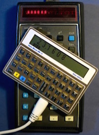
I originally wrote a Curve program for the HP-65 programmable calculator. Lately I have rewritten a program CurveP for a HP-15c or DM15 calculator. The HP-15c model is no longer available but a DM15 calculator is available from SwissMicros. This calculator is the size of a credit card and has more memory than the HP-15c. The calculator can communicate with a very nice HP-15c simulator from Torsten Manz. The advantage of this arrangement is that programs can be saved to and loaded from a computer. The simulator also allows extensive documentation to be saved in the program file. Programs are saved as plain text. An HTML summary file can also be created, for example, as CurveP.htm.
I have now written a new web page entitled SwissMicros DM15 Scientific Calculator.
HP-15c/DM15 Stray light curvature program - StrayLightP
StrayLightP is a program which corrects spectrophotometric data when stray light is present. It is an HP-15c or a DM15 scientific calculator program. The summary file StrayLightP.htm contains instructions and a program listing.
HP-15c/DM15 Mercury Analyser calibration curve program - HgCalP
A good calibration curve can be obtained using a simplified Dumarey equation - Reference: R. Dumarey, E. Temmerman, R. Dams, J. Hoste, Analyt. Chim. Acta 170, 337 (1985). The program HgCalP uses a temperature in degrees celcius to calculate the concentration of mercury in ng/ml in a calibration vessel. The summary file HgCalP.htm contains instructions and a program listing.
HP-15c/DM15 Regressions with a single entry of a data set - Stat4P
For general curve fitting Stat4P provides linear, logarithmic, power and exponential regressions with a single entry of a data set. This program is an adaptaton of software I wrote for a personal computer in 1984. For most statistical work a personal computer is best, but this program is good for a first look at experimental data. The summary file Stat4P.htm contains instructions and a program listing.
HP-15c/DM15 Toolkit - TVM, equation solving and curve fitting - ToolkitP
This Toolkit ToolkitP is intended to help a little with the use of laboratory equipment and processing the data produced. If income is earned the Toolkit can help with that too. The summary file ToolkitP.htm contains instructions and a program listing.
Conclusion
Some of these programs were used at DSIR Chemistry Division for many years. The flame emission curve fitting routines were particularly valuable when saline solutions were analysed as a wide range of concentrations could be handled in a single run. A colleague was even able to use the same equations to accurately model some oil viscosity data. The Stat4P regression program is recent.
Publications
- Algorithm for determinations of sodium, potassium, calcium and lithium over wide concentration ranges by flame emission spectrometry J. E. Patterson, Analytica Chimica Acta, Volume 107, 6 January 1979, Pages 201-209.
- Flame emission over wide concentration ranges. J. E. Patterson, Atomic spectrometry seminar, N Z Institute of Science Technicians, Wellington, August, 1979.
- Atomic Spectrometry Programs for the HP9815 Computing Controller. J. E. Patterson. Report CD2309, DSIR, Chemistry Division 1980.
- AAFLAME, programs for atomic absorption and flame emission. J. E. Patterson, IRL Report, March (1993).
JEP Related Links
AAFlame Software
AAFlame Documentation
DOSBOX
HP-15c/DM15 CurveP Software
SwissMicros
HP-15c simulator
SwissMicros DM15 Scientific Calculator
Programs
The following material is intended for use with computers rather than phones or tablets. The hp-15c Simulator at this stage only runs on a computer running Windows, Linux or macOS.
Clicking on any of the following links will cause a ZIP file to be downloaded. The extracted folder contains hp-15c program files, as well as documentation. I have included other programs that may be of interest.
Bike1 - 4 ProgramsBisecnewtP - Solver for hp programmable calculators
BisectionP - Solver for hp programmable calculators
Composite - 12 programs
CurveP - Curve Fitting
hp-15c Program Examples - 14 Programs
hp-15c Owner's Handbook - 14 Programs
hp-15c Advanced Functions Handbook - 7 Programs
hp-15c Matrix test routines - 2 Programs
hp-15c Owner's Handbook Matrix examples - 9 Programs
Maths1 - 8 Programs
Maths2 - 12 Programs
HgCalP - Calibrate Mercury Analyser
NewtonP - Newton Raphson Solver
Physics1 - 8 Programs
ReactanceP.15c - Reactance calculations, including inductor turns
SecantP - Solver for hp programmable calculators
Stat4P.15c - linear, logarithmic, power and exponential curve fitting
StraylightP - Stray light curve correction
ToolkitP - TVM, equation solving and curve fitting
Click the photos below to enlarge. Use the browser "back control" to return.
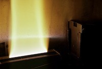
 Acetylene-Nitrous Oxide flame.
 AAFlame programs.
 AAFlame calibration.
 AAFlame calibration.
 SwissMicros DM15 calculator
